Fundamental Data Structures: Computational Complexity

Table of contents
What is the Computational complexity of an algorithm?
Computational complexity of an algorithm is a concept in computer science where we discuss the amount of resources that an algorithm needs to execute, or more precisely, its efficiency.
We usually focus on time complexity, where we consider the amount of time our algorithm needs to execute, and space complexity where we consider the amount of space our algorithm needs to run.
Having an efficient algorithm is great - it performs well, we minimize the number of resources we need, and our company is happy.
On the other hand, if we have an algorithm that utilizes a lot of resources to execute, in terms of both time and space, that means it requires more CPU power, more RAM, or something similar.
There is a financial aspect we need to consider when dealing with these things which means that this algorithm requires more money in the end, which could represent an issue.
Then we would probably get a task where we would have to analyze the algorithm to see if it can do better.
In its core, when it comes to the computational complexity of an algorithm, or the algorithm analysis, it all comes down to answering the following question:
How does our algorithm scale if we keep giving more and more data to it?
Now, to be more precise this is what asymptotic algorithm analysis is about.
In mathematical analysis there is a concept of asymptotic analysis, which is essentially a way of describing a certain behaviour of a function.
What kind of behaviour?
Given a function f(n), what is the value that the function approaches, as the input n approaches a particular value.
So asymptotic algorithm analysis is basically asymptotic analysis but in the context of algorithms.
When analysing algorithms, there is a need to come up with a function that represents the description of how, in general, the algorithm scales when the input size gets arbitrarily large.
You might have noticed that I highlighted in general.
Why did I do that?
If we were to come up with a precise and detailed function, we would have to take into account a lot of things: different computer architectures, different operating systems, various programming languages - compilers/interpreters, and so on.
Perhaps different computer architectures do not handle basic arithmetic operations the same, and possibly different operating systems do not handle memory allocation/deallocation the same. Perhaps different programming languages do not handle loops the same (theoretically), and so on.
So, if we were to make a rigorous analysis of an algorithm, we would have a rough time achieving this.
How do we approach this?
In short - we try not to worry about details.
We can rely on something which in the theory of computer science is called RAM - Random Access Machine. We could say that It is an abstract machine or a platform that we use as a model when analysing algorithms. It has the following properties:
- Basic arithmetic operations such as addition, subtraction, multiplication, division, and basic logical operations take precisely a one-time step
- Loops and subroutines are not straightforward operations, rather they are a composition of simple operations, so they take multiple-time steps
- Memory access takes precisely a one-time step, and we do not have to worry if the data is in the main memory or on the disk
Using this model of computation, we can come up with a machine undependable description of time or space complexity of an algorithm.
What is the Big O Notation?
When discussing the time or space complexity of an algorithm, we mostly refer tothe worst-case scenario - the “Big O Notation” - how our algorithm will perform if we give it the most significant amount of data.
There is also Big Omega Notation which represents the best-case scenario as well as Big Theta Notation which represents the average-case scenario, but in this post we will focus only on the Big O Notation.
Additionally, we will only focus on the time complexity.
We could say that Big O is this expression of the runtime of our algorithm in terms of how quickly it grows as the input gets arbitrarily large, or as we said earlier - how well it scales.
But, why would we care about the worst case? Is this not a bit counterintuitive?
In his book The Algorithm Design Manual, Steven Skiena tries to answer this question through an interesting illustration.
He says that we should imagine a scenario where we bring n dollars into a casino to gamble.
The best case scenario would be that we walk out owning the place - which is possible but extremely unlikely to happen.
The worst case scenario is that we lose all n dollars, which is unfortunately more likely to happen and can be calculated.
The average case in which the bettor loses around 90% of the money that he brings to the casino is difficult to establish and is subject to debate.
Then he asks himself what average means in the first place.
Unlucky people lose more than lucky people, so how to define who is more fortunate than who, and by how much?
So, we could avoid these complexities by considering only the worst case scenario.
After all, if we come up with the worst-case scenario that represents an upper bound - we guarantee that our algorithm will not perform worse than that, only equally, or better.
Imagine that you have an algorithm whose worst-case scenario time complexity is represented by function f(n) = 215n^2 + 33n + 7092 ?
In the worst-case scenario, this algorithm would take 215n^2 + 33n + 7092 steps to execute.
What Big O does is the following:
It says that this function is too detailed and that we can generalise it by following these steps:
- Drop constant factors
- Drop lower-order terms
Why do we do this?
Constant factors are the things that depend on environment details, whether the environment is specific computer architecture, operating system, or a programming language. If we do not want to focus on these particular things but rather be generic, we should not focus on them.
Lower-order terms become irrelevant when we focus on the larger (and eventually infinite) amounts of data - and this is what we want. We want our algorithm to perform well on large amounts of data - this is where algorithm ingenuity lies. After all, in software engineering, it is pretty much all about the data.
Let us take a look at our function f(n) = 215n^2 + 33n + 7092.
If we were to drop constant factors:
f(n) = 215n^2 + 33n + 7092
We would get this:
f(n) = n^2 + n
Why did we do this?
Remember that we said that Big O cares about the runtime but when the input gets arbitrarily large?
If our input, that is n, gets bigger and bigger, at some point, it will get so big that multiplying it by 215, and by 33 or adding 7092 does not have a significant effect.
The next step would be to drop lower-order terms:
f(n) = n^2 + n
And why do we do this?
Because n^2 is the dominant term out of the two, that is, n^2 is the function that grows faster than the function n, as the input gets bigger and bigger.
Therefore, n is the lower-order term and eventually will not have a significant impact.
At the end we are left with this:
f(n) = n^2
This function f(n) = n^2 would represent the Big O or the worst-case scenario time complexity of our algorithm.
We might also use the vocabulary where we say that our algorithm is on the order of n^2 - O(n^2), which means that it does not necessarily have to be n^2. Instead it tends to be n^2.
And that is essentially what Big O is about.
Big O buckets our algorithms into specific classes based on their worst-case time complexity (runtime), by dropping constant factors and lower order terms.
Like with most things, I believe, there is a specific mathematical background you need to consider here.
However, in this blog post, we will not dive deep into the mathematical formalism of Big O, so do not worry.
We mentioned Big O classes.
Let us look at the most common ones, starting from the best to the most undesirable ones.
O(1) - Constant Time Complexity
Any algorithm that is O(1) executes in constant time, that is, it always executes a fixed number of operations, regardless of the input size.
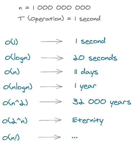
Let us presume that a single operation takes 1 second.
If we have an input of size 10, our algorithm will take 1 second to execute.
If we have an input of size 1 000 000 000, our algorithm will still take 1 second to execute.
Returning the first element of an array.
O(log n) - Logarithmic Time Complexity
Since logN is a function that grows slowly, any algorithm that is O(logN) is pretty fast.
These algorithms usually do not have to process the whole input; they usually halve the input in each stage of their execution.
You can think of these algorithms in this way as well:
Every time the size of the input doubles, our algorithm performs one additional operation/step - which is a pretty good scaling.
If we have an input of size 1 000 000 000, and a single operation takes 1 second, our algorithm would take 20 seconds to execute.
O(n) - Linear Time Complexity
Any algorithm that is O(n) has its runtime proportional to the size of the input.
This means that these algorithms process each piece of the input, meaning they have to look at each element/item once.
If the size of the input doubles, the number of operations/steps doubles.
If we have an input of size 1 000 000 000, and a single operation takes 1 second, our algorithm would take 11 days to execute.
Printing all elements of an array.
O(n logn) - Linearithmic (Superlinear) Time Complexity
Depending on the literature n logn time complexity is referred to as linearithmic, superlinear or log-linear.
If we have an algorithm that is O(n logn), that means that we might have an advanced sorting algorithm such as Merge sort.
If we have an input of size 1 000 000 000, and a single operation takes 1 second, our algorithm would take 1 year to execute.
O(n^c) - Polynomial Time Complexity
An algorithm that has polynomial time complexity - n^c where c is larger than 1, is generally slower than an O(n log n) algorithm.
When c equals 2, for example, we are talking about an algorithm that has quadratic time complexity, and these algorithms usually process all pairs of n elements.
If the size of the input doubles, the number of operations/steps, required by that algorithm, quadruples.
If we have an input of size 1 000 000 000, and a single operation takes 1 second, our algorithm would take 32 000 years to execute.
Example: One of the elementary sorting algorithms, such as Insertion sort.
O(c^n) - Exponential Time Complexity
An algorithm that is O(c^n) is better to be avoided, if possible.
These algorithms are really slow and are impractical for large data sets.
Algorithms that are O(2^n) are a common representation of this Big-O class, and they generally occur during the processing of all subsets of n items.
If the size of the input increases by one, the number of operations/steps, required by that algorithm, doubles.
If we have an input of size 1 000 000 000, and a single operation takes 1 second, our algorithm would take eternity to execute.
O(n!) - Factorial Time Complexity
An algorithm that is O(n!) is, again, better to be avoided.
These algorithms are also extremely slow, even slower than exponential ones and cannot be used for large data sets.
They generally occur when processing all combinations of n items.
If we have an input of size 1 000 000 000, and a single operation takes 1 second, our algorithm would take even more than eternity to execute.
Example: the travelling salesman problem.
Fun fact:
O(∞) - Infinite Time Complexity
An algorithm that is O(∞) will take, well, infinity to execute.
You might not believe this, but there is actually an example of this algorithm called Stupid Sort that takes an array, randomly shuffles it, and checks to see whether it is sorted.
If not, it randomly shuffles it again and checks whether it is sorted. And again and again, potentially up to the infinity.
Take a look at the picture above.
When we gave examples of how long it would take for each of these algorithms to execute, we got some interesting values such as 32 thousand years or eternity.
We intentionally used 1 second for each operation and 1 000 000 000 for the size of the input in order to end up with these values, just to show how drastic and dramatic the difference between these classes can be.
Finally, we can take a look at the difference between these Big O classes:
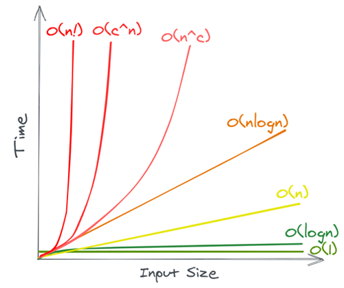
As we can see, constant time complexity and logarithmic time complexity are considered good, and we should aim for these if possible.
Linear time complexity, as well as linearithmic time complexity are average and we can get away with these.
Some of the best sorting algorithms are actually O(n log n), so we can not do better than this.
Polynomial, exponential, and factorial are considered very bad, and we should avoid these, if possible.
How to Determine The Big O?
So far, we have seen what Big O is, and what some of the most common Big O classes are.
But how do we actually determine which of these classes our algorithm belongs to?
Our algorithm is represented by a sequence of different statements:
{ StatementOne; StatementTwo; StatementThree; . . . StatementN;}
The statements could either be simple statements such as assignments, function calls, returns, and so on.
You could think of these as simple operations.
There are also compound statements such as conditionals, loops, blocks - which are, again, just a sequence of statements, and so on.
In order to get the total amount of steps that our algorithm needs to execute, we have to sum up the number of steps of each of these statements:
- Simple Statements
- Compound Statements
What are Simple Statements?
Let us presume that each statement is a simple statement - a simple operation.
In that case, the worst-case time complexity of each statement would be constant - O(1).
Our algorithm itself would then be - O(1).
Why? Because, when we sum up constants, we end up with a constant.
What are Compound Statements?
With compound statements, it is a bit different.
If the statement is a conditional such as if-else:
if(condition) { firstBlock}else { secondBlock}
Based on the condition, either firstBlock or secondBlock is going to execute.
Since Big O represents the worst-case time complexity, we need to take into account the block that has the worst time complexity out of the two.
If, for example, firstBlock is O(1) and secondBlock is O(n), then we would take into account secondBlock.
In that case, the overall time complexity would be O(n).
If the statement is a loop such as for loop:
for(i in range 1 to n) { someBlock}
This loop is going to execute n times; therefore, someBlock is going to execute n times as well.
If the case is that someBlock represents purely a sequence of simple statements, meaning that someBlock is O(1), then the overall time complexity is O(n).
Why?
For each n iterations of the loop, someBlock gets executed - O(n) * O(1) = O(n).
If the statement is a nested loop:
for(i in range 1 to n) { for(j in range 1 to n) { someBlock }}
For each n iterations of the outer loop, the inner loop makes n iterations as well.
Therefore, someBlock is going to execute n*n, which means that the overall time complexity is O(n^2).
However, if the case is that the inner loop makes m iterations, the overall time complexity would be O(n * m).
With both cases there is an assumption that someBlock is a sequence of simple statements.
If the statement is a function call:
In case that a statement represents a function call, the complexity of that statement is actually the complexity of the function.
Let us say that we have a function someFunction(input) for which we have previously determined that it is O(n), meaning that it takes linear time to execute.
for(i in range 1 to n) { someFunction(i)}
For each n iterations of the loop, someFunction(i) gets called. Since each call of the someFunction(i) is O(n), what we get is the O(n^2) overall time complexity.
Practical Example
To conclude, let us try to analyze the following algorithm to see what its worst case time complexity is.
Let us say that we have an algorithm that takes an array of unsorted integers and returns the smallest integer.
9 public int findSmallestInteger(int[] arrayOfIntegers) { 10 int smallestInteger = Integer.MAX_VALUE;1112 for (int integer : arrayOfIntegers) {13 if (integer < smallestInteger) {14 smallestInteger = integer;15 }16 }17 18 return smallestInteger;1920 }
Keep in mind that we do not have to worry about the exact amount of time needed for variable declaration and assignment, executing the if condition, variable reassignment and so on since these are considered to be simple operations that take exactly one time step - we rely on the RAM model of computation.
On line 10 we have 1 operation.
On lines 12 - 16, we have a loop that executes n times where n is the number of elements inside our array.
On line 13 we have an if condition - 1 operation.
How many times will line 14 execute?
Well, in the worst case the smallest integer could be at the end of our array so it will execute each time - therefore 1 operation.
On line 18, we have 1 operation.
So we have 2 operations inside and 2 operations outside of our loop, which leaves us with 2*n + 2.
If we were to drop constants 2*n + 2, we would get n.
Finding the smallest element in an unsorted array is O(n).
In other words, finding the smallest element in an unsorted array has linear worst-case time complexity.
Now that we have explained the concept of Big O a bit better, we can go back to the next data structure.
In the next blog post, I am going to talk about linked lists.